
A stability analysis of a Hall-HÚroult cell requires a detailed calculation of the Lorentz forces in the metal pad. Factors that affect the calculation of these forces such as the current density distribution and the presence of ferromagnetic materials are reviewed.
Three dimensional thermo-electro-magnetic models of a typical Hall-HÚroult cell are developed using Revisions 4.4A and 5.0 of ANSYS. The models represent increasing levels of complexity to evaluate the effects of the accuracy of the current density distribution and of the ferromagnetic potshell. The problems associated with developing a large multi-field model are discussed.
INTRODUCTION
For more than 100 years, the Hall-HÚroult process has been and continues to be the only commercially viable method for making aluminum. The design and operation of a Hall-HÚroult reduction cell, the facility used to produce aluminum, requires a detailed understanding of the thermal, electrical and magnetic behavior of the cell as well as the stresses due to thermal gradients and carbon swelling.
Several finite element models have been developed over the last 10 years to study the cell behavior. This paper will focus on the calculation of the electric and magnetic fields within the cell and the Lorentz forces they generate in the liquid metal. Factors that affect the calculation of these quantities will be reviewed and the results for the analysis of a typical cell will be presented.
THE HALL-H╔ROULT REDUCTION CELL
Aluminum is produced from alumina (A1203) by reduction, a chemical term meaning the removal of oxygen. The process takes place in electrolytic cells known as pots. A typical pot is shown in Figure 1. A pot contains molten electrolyte (bath) in which alumina is dissolved and from which aluminum is produced. Immersed in the bath are rectangular carbon anodes that act as the positive electrode. Electrical current passing from the anode through the electrolyte to the metal pad, which acts as the cathode, reduces the alumina molecules into aluminum and oxygen. The oxygen reacts with the anode carbon to form carbon dioxide. The aluminum, being heavier than the electrolyte settles to the bottom of the pot. The molten electrolyte and aluminum are contained in a steel shell lined with refractory brick and carbon blocks surrounded by a lamming mix (see Figure 1). A layer of frozen electrolyte (freeze) forms on the sides of the pot to protect the side carbon block and mix.
Figure 1: Typical Hall-HÚroult cell
Typically, a smelter consists of one or more potlines each having 100-200 pots. Pots are connected in series through a network of aluminum busbars shown in Figure 2. Risers feed electrical current to an anode busbar from which anode rods carry the current to the anode carbon. Within the cell, the current flows through the bath and the metal pad into the cathode carbon and exits the cell via steel collector bars embedded in the cathode carbon. The collector bars are connected to a common busbar that connects to the riser of the next pot.
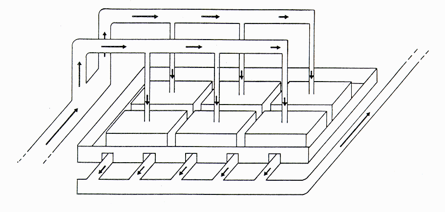
Figure 2: Typical arrangement of busbars
EVALUATION OF POT PERFORMANCE
The stability of a cell during operation depends on the magnetic and electric fields within the metal pad and bath. According to Davidson and Boivin [1], the change in the electric and magnetic fields as a result of a disturbance in the bath/metal interface will transfer electro-magnetic energy into mechanical energy leading to a standing wave within the pot. The existence of a standing wave leads to an increase in the energy consumption of the cell and a reduction in current efficiency due to metal Deoxidization. It may also short circuit the cell.
Figure 3 depicts the steps necessary to perform a stability analysis of a pot and evaluate pot performance. The first step is to define the cell geometry and calculate the current density within the cell and the surrounding busbars. This distribution is then used to calculate the magnetic field. Note that the effects of the ferromagnetic steel shell need to be considered in the magnetic field analysis. The magnetic and electric fields are used to calculate the force field in the metal pad and bath. The next step is to calculate the flow pattern of the metal pad and bath and the shape of the bath/metal interface using the force field distribution. Finally, the velocity profile, magnetic and electric field distributions, and the shape of the bath/metal interface are used to perform a stability analysis of the pot.

Figure 3: Hierarchy of steps required for stability analysis
ANALYSIS CAPABILITIES REQUIRED FOR THE CALCULATION OF THE MAGNETIC FIELD
ANSYS based thermo-electro-magnetic modeling is highlighted in Figure 3. Thermo-electric models (not shown in Figure 3) are used to predict the shape of the freeze profile which is part of the geometry definition of the bath and metal pad. Details of these models were presented at earlier ANSYS conferences [2,3].
The characteristics of a reduction cell that significantly affect the magnetic field solution can be grouped into four areas:
| 1. | The conductors (collector bars and busbars) carrying current to and from the cell give rise to magnetic fields inside and outside the shell. Although some conductors are far away from the cell, they can have significant contributions chat must be considered. This has implication on the size of a model and the ease with which these source currents can be incorporated in the model. |
| 2. | The magnetic field is an open boundary problem. Hence, far field effects must be adequately represented. Closed boundary approximations using repetitive symmetry conditions and other solution techniques may result in large discrepancies between calculated and measured values [4]. |
| 3. | The presence of the ferromagnetic shell with holes significantly modifies the magnetic field inside the shell. Appropriate solution techniques are necessary to cope with the nonlinear permeability of the shell and the multiply connected domains created by the holes. |
| 4. | The presence of distributed currents within the cell must be taken into account. In particular, two factors need to be considered. The first is the presence of horizontal currents due to the bias towards side exit. These produce horizontal components of the force field which affect the metal circulation pattern. The second factor is the local impact of the freeze profile on the current distribution in the metal, which may even result in the reversal of the horizontal current. |
Given the above, it is clear that ANSYS has several advantages to offer. In particular, two ANSYS features are noted:
1. Coupled Field Analysis
This capability is advantageous in three areas. First, thermo-electric coupling allows for a detailed calculation of the current density and the shape of the freeze profile [2,3]. The temperature dependent material properties can be incorporated in the model as well as all the thermal and electrical boundary conditions on the cell. Second, the electro-magnetic coupling allows for an automatic transfer of the source currents calculated in the thermo-electric analysis to the magnetic field analysis. Finally, the same model can be used to calculate the thermal, electric and magnetic field solutions.
2. Magnetic field Solution
ANSYS offers four options to calculate the magnetic field: Three Scalar Potential formulations (Reduced RSP, Difference DSP and Generalized GSP) and a Vector Potential formulation (VP). For the problem at hand, the GSP formulation is the only viable option for the following reasons.
| . | VP requires that the current source be meshed in the model as part of the overall geometry. This gives rise to a horrendous meshing job (see Figure 9). Furthermore, the VP uses three degrees of freedom per node resulting in large model sizes and wavefronts and hence long processing times. Scalar potential formulations uncouple the source current mesh from the magnetic field mesh, i.e. you can mesh each part separately. Furthermore, only one degree of freedom per node is active thus reducing the problem size and running time. |
| . | The RSP formulation is limited by cancellation errors when current and iron are present. The DSP formulation is limited to singly connected iron regions. Cuts in the iron region would have to be introduced to use the DSP formulation. The GSP formulation can handle multiply connected domains without the need for cuts and without the problem of cancellation errors. |
Other ANSYS capabilities which were found advantageous include the nonlinear material capabilities with a robust solution procedure to handle them; the Parametric Design Language (APDL) which allows for the development of generic parametric models (thus reducing the model development time) and facilitates the exporting of results for use in other applications; and the extensive pre- and post-processing capabilities for developing models and viewing results.
MODEL DEVELOPMENT
The goal of the present study was to evaluate the use of ANSYS for calculating the force field in the metal pad and the feasibility of incorporating all the factors described in the previous section. Some simplifying assumptions were made to make the problem manageable. The first was to ignore the detailed distribution of the ferromagnetic material by assuming a simple rectangular box. The second was to limit the size of the air surrounding the shell. Rather than use the total volume that encompasses all the busbars, the air boundaries were set at a reasonable distance from the shell. The impact of these assumptions can be evaluated in future studies.
Two analyses were planned that took advantage of existing models and modeling capabilities. The first was an electro-magnetic model which ignored thermo-electric coupling with the assumption of constant electrical resistivity (calculated at pre-defined temperatures) for the various components. Also, an approximate freeze profile was used. The second analysis examined the thermo-electro-magnetic coupling with a previously calculated exact freeze profile. In both cases the following steps were involved:
| 1. | Develop model geometry and boundary conditions. |
| 2. | Calculate the electric field solution and the corresponding current density. |
| 3. | Calculate the Lorentz force in the metal pad. Ignore the shielding effects from the steel shell. |
| 4. | Calculate the Lorentz force in the metal pad. Include the shielding effects from the steel shell. |
The solution steps (2 to 4) represent increasing levels of complexity and resource requirements.
The two analyses allow for evaluation of the impact of using an accurate freeze profile and 3D solid elements for the busbars and risers, and the shielding effects due to the steel shell. Because the models are parametric, several sensitivity studies can be easily performed. In particular, the benefit of adding more shielding and the assumption regarding the size of the volume of the surrounding air can be evaluated by changing parameter values in the model. The contribution of busbars far away from points of interest can be evaluated by unselecting elements representing these segments. Note that each change requires a new solution and hence processing time becomes increasingly important.
The first analysis was successfully completed. Unfortunately, computing resources and time constraints prevented the completion of the second analysis prior to the publication of the conference proceedings. As a result, the following discussion will focus on the development of both models and present results from the first analysis only.
ELECTRO-MAGNETIC MODEL
Figure 4 shows a model of the inside of the cell. It includes the bath and metal pad, the immersed anode carbon, the cathode carbon and the steel collector bar. More than 35,000 elements with 40,000 nodes were used. The mesh was created using a generic ANSYS model (called CURDEN) developed to study the electric field in the cell. CURDEN is a general purpose ANSYS parametric model developed for Alcan by Compusim. It automatically creates and meshes cell geometry, applies the boundary conditions, calculates the current density in the model and prepares custom results tables and plots. The user prepares an input file of parameter values that describe the particular design and simply runs CURDEN. The model is very versatile allowing for any number of cathode blocks with one or two collector bars, any number of anodes, a variable freeze profile, a variety of boundary condition options at the bar ends and several other features. The geometry part of CURDEN was used to generate the mesh shown in Figure 4.
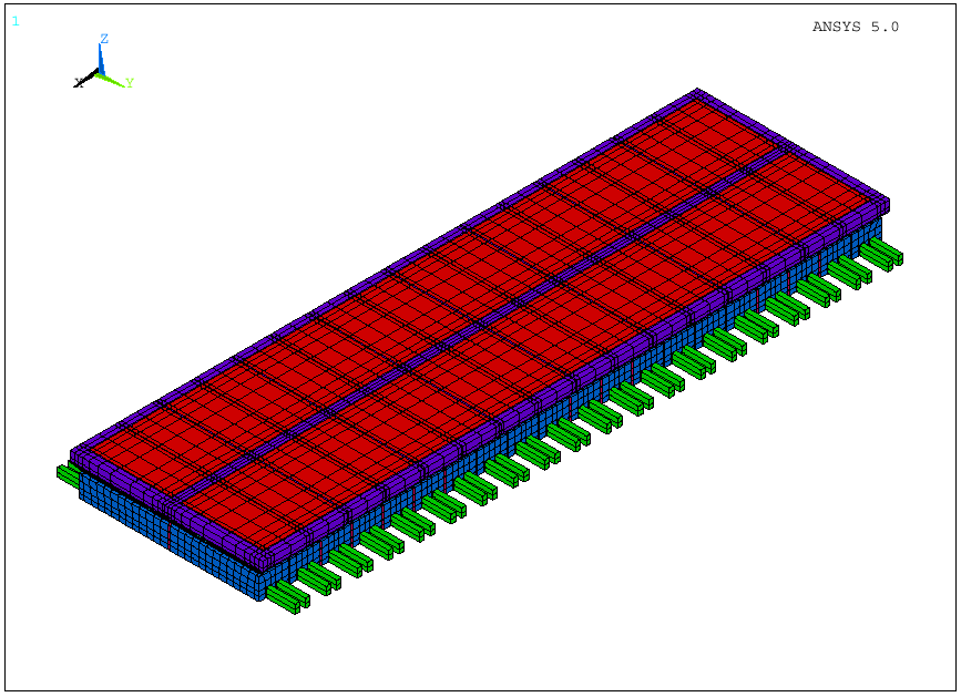
Figure 4: Finite element mesh of electro-magnetic model: Electric field model inside the shell
A portion of the busbar network surrounding the pot is shown in the zoom plot of Figure 5. The conductors shown are line elements plotted using the /ESHAPE command in ANSYS. This segment of the model was created using a custom translator of existing data used by Alcan's special purpose in house programs. Close to 6,000 elements with 3,000 nodes were used to model this segment. The full busbar network was modeled.
Figure 6 shows a zoom plot of the full model. It highlights the steel shell and the surrounding air which were meshed using macros developed to enhance CURDEN's features. The model is parametric allowing for changing the size and mesh density of the air volume and the position and size of the steel shell. The full model consisted of 131,000 elements with 145,000 nodes.
Figures 7 and 8 show contour plots of the force field in the middle of the metal pad with and without shielding from the shell. A rigorous analysis of the results is not part of this study. However, it was sufficient to demonstrate that the values of the magnetic field are comparable to measured values and to those calculated by other tools.
The model was developed on an HP720 workstation with 64 MB of RAM using Revision 5.0 of ANSYS. The database file for the full model was close to 100 MB. The solution was processed with Revision 5.0A on a CRAY C90 in three steps. The current density was calculated first. It was used as input to solve the unshielded and shielded magnetic field. The total CPU time was slightly over 11 hours. In order to process the model in core it was necessary to specify 336 MB of work space for ANSYS. The final database files for the unshielded and shielded solution were 181 and 303 MB respectively.
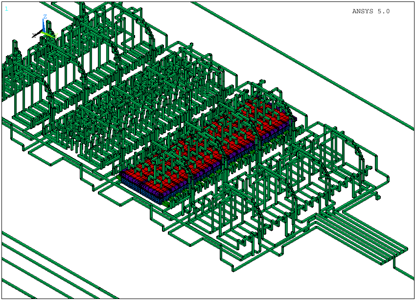
Figure 5: Finite element mesh of electro-magnetic model: Busbar system around the cell

Figure 6: Finite element mesh of electro-magnetic model
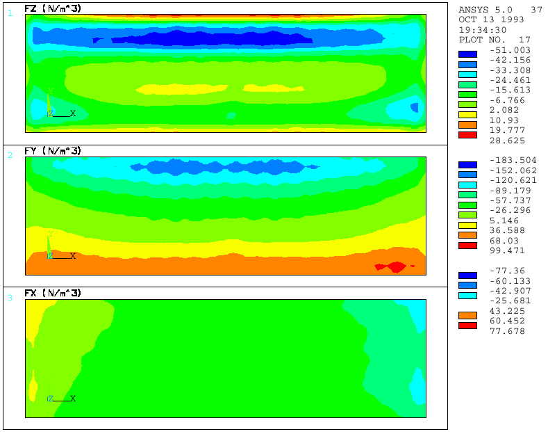
Figure 7: Force field solution at the middle of the metal pad - Unshielded case

Figure 8: Force field solution at the middle of the metal pad - Shielded case
THERMO-ELECTRO-MAGNETIC MODEL
Figure 9 shows the thermo-electric part of the second analysis. The model shown differs from that presented in Figure 4 in two areas. First, an "exact" freeze profile was used to define the geometry of the bath and metal pad. The freeze profile was calculated using a quarter thermo-electric model developed specifically for that purpose (see references 2 and 3 for a detailed description of the model and the calculation of the freeze profile). The second difference was the detail with which the risers, busbars, anodes and anode rods were modeled. In this case 3D solid elements were used.
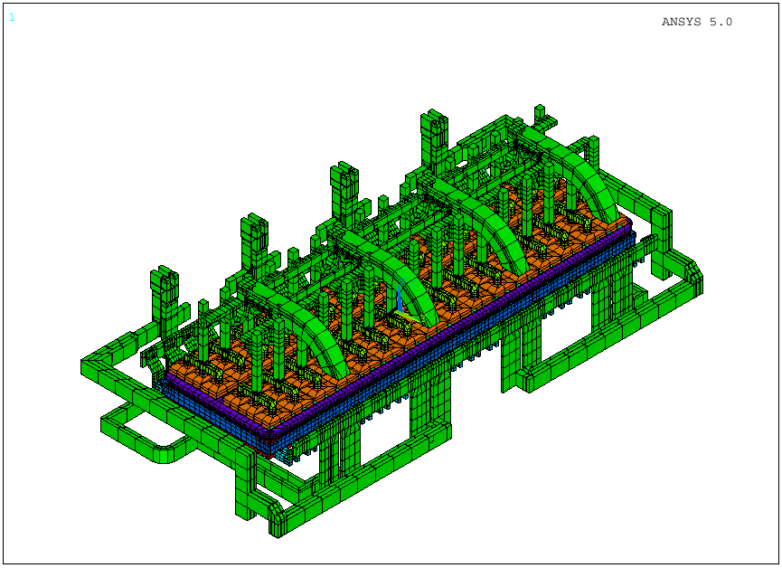
Figure 9: Finite element mesh of thermo-electric model
The model shown in Figure 9 was developed using Revision 4.4A of ANSYS. It is the amalgamation of six separate ANSYS models in one. The six models are: a quarter cell model for calculating the freeze profile, four models of the busbars around the cell and a detailed model of one quarter of an anode. Each model was run separately to calculate the temperature and voltage solution. Results were compared to measured values to verify the models. The full model was then created by first mirroring the quarter cell model twice. Next, the quarter anode model was mirrored twice to create a full anode and then repeated as needed to create the full anode panel. These models along with the busbar models were combined into one by issuing a CDWRITE command for each and then using /INPUT commands to read the FILE28s in the final model. The challenge was to make sure that the coordinate systems and the coordinates of the interface nodes in each model were the same so that everything fell in place when all models were combined. The versatility of the ANSYS commands and its capabilities were very much appreciated.
Once the model was in place, a thermo-electric solution was performed to calculate the current distribution. To reduce the problem size, the temperature solution from the anode run and the quarter cell was prescribed as nodal temperatures. The temperature solution from the quarter models was written as NT commands using *CFWRITE. Appropriate generation values were specified to create the data for the mirrored segments. Convection surfaces were defined on the busbars to complete the definition of the boundary conditions. Note that temperature dependent material properties were specified for all materials. Also, temperature dependent equivalent surface film coefficients that included convection and radiation effects were used. These two factors account for non-linearity in the model.
A solution was performed on an HP720 workstation. The non-linear solution required 11 iterations to converge. The total elapse time was 12 hours. The results of the analysis compared very favorably with the solution from each separate model. This confirmed that the combination of all models together did not create any errors. Furthermore, it confirmed that assumptions made in each model vis-Ó-vis its interaction with adjacent parts were adequate.
The 4.4A model was ported to Revision 5.0 and expanded to add the rest of the busbar network, the steel shell and the surrounding air. The magnetic solution was not performed due to limited computing resources.
DISCUSSION
The successful solution of the electro-magnetic problem demonstrated the feasibility of using ANSYS to calculate the force field in an aluminum reduction cell. There were no problems in developing the model and running the solution. The coupled field analysis worked very well. The Generalized Scalar Potential formulation could handle the ferromagnetic material and the multiply connected domain in the steel.
The biggest problem was the resources needed to process the model. Recall that it took more than 11 CP hours to run the model on a CRAY C90 and 336 Mbytes of ANSYS workspace to run it in core. A close look at the running time for each step estimated from the ANSYS output file (Table I) indicates that considerable time was spent processing the BIOT command (32% of total running time). Possible improvements in the calculation performed by this command would definitely impact total solution time.
| Electric field solution | 1800 |
| Magnetic field solution (Unshielded) | 4300 |
| À BIOT command | 2500 |
| À All other | 1800 |
| Magnetic field solution (Shielded) | 33800 |
| À BIOT command | 9000 |
| À Non-linear solution (Step 1; 9 iterations) | 8000 |
| À Non-linear solution (Step 3; 10 iterations) | 12100 |
| À Formulation of element matrices (per iteration) | 1100 |
| À Matrix triangularization (per iteration) | 300 |
The second area where considerable time was spent was in processing the non-linear solution due to the presence of the ferromagnetic material. Approximately 30% of the total CPU time was spent in recalculating the element matrices. Yet only the elements representing the steel shell are non-linear and they are only 7% of the elements in the model. Significant savings in processing time may be achieved by reducing the element reformulation time of linear elements. In fact, such an improvement would be beneficial in other non-linear problems where linear elements are used.
Because of the extensive computing resources required for the analysis, it is not feasible at this point to perform sensitivity studies using such models. Advances in workstation performance as well as enhancements to ANSYS are needed before full scale sensitivity analyses can be performed.
CONCLUSION
The work described above has demonstrated the viability of calculating the force field in an aluminum reduction cell using ANSYS. It is possible to account for all the complexities inherent to the calculation.
The computing resources required to process the model are considerable which prohibits its use in the near future. Advances in computing performance of workstations and enhancements to ANSYS would make it more feasible to run the model and perform the necessary sensitivity studies for design purposes.
ACKNOWLEDGMENTS
The authors would like to thank Mr. John Twerdok and Mr. Lou Muccioli of Swanson Analysis Systems and Cray Research for providing the resources to process the magnetic field model. Also, we would like to thank the management at Alcan's Arvida Research and Development Center for allowing publication of this work.
REFERENCES