USING A STEADY STATE MODEL OF AN ALUMINUM REDUCTION CELL
TO INVESTIGATE THE IMPACT OF DESIGN CHANGES
Marc Dupuis GéniSim 3111 Alger St., Jonquière, Québec, Canada G7S 2M9 email:
Imad Tabsh
CompuSIM Inc.
1003 D 55 Avenue N.E., Calgary, Alberta, Canada T2E 6W1
email: tabshi@compusim.com
ABSTRACT
A program was developed to model the steady state behavior of an aluminum reduction cell. The program simulates the electrolytic process by solving the heat and mass balance equations that characterizes the behavior of eleven chemical species in the system. The steady state convergence scheme has been designed in such a way that it can solve for any of the 18 main parameters having defined the 17 others. Furthermore, those 17 parameters can be defined using probability functions. As a result, the output parameter will also be presented in the form of a probability function. The program is a PC based Windows® application that takes full advantage of the Windows user interface. This paper describes the implementation of that model and also presents examples of practical applications.
INTRODUCTION
The design and operation of an aluminum reduction cell is a complex task requiring a detailed understanding of the behavior of the cell. In a previous publication[1], it has been demonstrated that a computer program can successfully simulate the dynamic behavior of a reduction cell. Such a program is quite valuable as a teaching tool that enables the user to rapidly develop more insight into the behavior of the cell.
Such a dynamic model can also be used to investigate the impact of alternative operating practices or control strategies in order to improve the success rate of potline improvement projects.
The third application of the model that comes to mind is the analysis of the dynamic behavior of new or retrofit cells. This is in the context of performing feasibility studies to quickly establish design target for the anode and cathode voltage drop as well as the anode panel and cathode lining heat dissipation. Obviously, even before studying the dynamic behavior, the new design must first provide an acceptable steady state solution.
Although a steady state model was already part of the full dynamic model package, this paper presents an enhanced version of the steady state solver to be used for risk assessment of design alternatives.
PROGRAM OVERVIEW
Compared to the full dynamic model presented before[1], the steady state model subset only requires a Process Model to simulate the electrolytic process that characterizes the pot behavior. The heat balance equation over the system of interest is the only constitutive equation that needs to be solved, the system of interest being defined as the liquid zone (bath and metal) and the solidified ledge. The thermal balance of the system is obtained by evaluating the internal heat generation and the heat loss from the system. In steady state mode, these two must be equal by definition.
Internal heat
The internal heat is evaluated by computing the voltage break down. The task is performed in modules each of which solves for a component of the voltage breakdown using submodels. A submodel consists of one or more equations that define the variable(s) in the module. The program has built-in equations for each submodel based on data in the literature [2-8]. In addition, the user can customize the equations of a submodel using the internal variables available in the simulation.
The modules that define the internal heat are:
| · Bath composition | · Bath voltage | · Bath resistivity | |||
| · Electrolysis voltage | · Bath liquidus | · Current efficiency | |||
| · Equivalent voltage to make metal |
Heat loss
Evaluation of the heat loss is simplified by assuming that the heat produced in the system can escape from four different surfaces: the anode panel, the cathode panel, the ledge adjacent to the bath layer and the ledge adjacent to the metal layer.
A constant thermal resistance is assumed for the cathode and anode panels. Thus, the heat loss from these two surfaces is only a function of the difference between the operating temperature and the ambient temperature in the potroom. The anode panel includes everything above the top surface of the bath while the cathode panel includes everything below the level of the collector bars.
The global thermal resistance adjacent to the ledge is a function of the thermal conductivity and the thickness of the ledge, mix and side carbon as well as the heat transfer coefficient of the convective film on the potshell surface.
Solution strategy
The constitutive equation that needs to be solved is:
Internal heat - Heat loss = 0 (1)
The solution strategy is to find the root of the above equation by selecting one "variable" for the standard Newton-Raphson root search algorithm:
f(x) = 0 (2)
Any of the 18 main cell input parameters appearing in the Table I may be selected as "variable" for the root search. This means that the user may select any one of those 18 parameters as an output variable and converge on a steady state solution.
Table I - List of possible root search "variable"
| Amperage of the cell (kA) | Length of the anodes (m) | |
| Anode to cathode distance or ACD (cm) | Width of the anodes (m) | |
| Concentration of excess aluminum fluoride (%) | Heat loss of anode panel (kW) | |
| Concentration of dissolved alumina (%) | Anode voltage drop (mV) | |
| Concentration of calcium fluoride (%) | Length of the cell cavity (m) | |
| Concentration of lithium fluoride (%) | Width of the cell cavity (m) | |
| Concentration of magnesium fluoride (%) | Heat loss of the cathode bottom (kW) | |
| Height of bath (m) | Cathode voltage drop (mV) | |
| Height of metal (m) | Cell operating temperature (°C) |
SIMPLE "WHAT IF" SCENARIO APPLICATIONS
This is a very practical tool to test the feasibility of changes in cell design. For demonstration purposes, a case study based on a prototype cell operating at 300 kA is presented [9]. Using the information available in the reference and assuming some values, 17 of the main parameters were defined as shown in table II:
Table II - Cell parameters values from reference 9
| Amperage of the cell (kA) | 300 | Length of the anodes (m) | 1.6 | |
| Concentration of excess aluminum fluoride (%) | 8.5 | Width of the anodes (m) | 0.8 | |
| Heat loss of anode panel (kW) | 235 | |||
| Concentration of dissolved alumina (%) | 2.0 | Anode voltage drop (mV) | 300 | |
| Concentration of calcium fluoride (%) | 3.0 | Length of the cell cavity (m) | 14.1 | |
| Concentration of lithium fluoride (%) | 0.0 | Width of the cell cavity (m) | 4.05 | |
| Concentration of magnesium fluoride (%) | 0.0 | Heat loss of the cathode bottom (kW) | 90 | |
| Height of bath (m) | 0.20 | Cathode voltage drop (mV) | 300 | |
| Height of metal (m) | 0.18 | Cell operating temperature (°C) | 975 |
ACD, the only undefined input parameter, was selected as the output variable for the Newton-Raphson root search algorithm. Assuming a value of 4.0 cm as the initial guess, the convergence proceeded as follows:
| Table III - Convergence behavior | Table IV - Steady state results | ||||||
| x | f(x) | ACD (cm) | 4.9951 | ||||
| 4.0000000 | -79.4145 | Cell voltage (V) | 4.27 | ||||
| 4.9773096 | -1.39511 | Current efficiency (%) | 91.6 | ||||
| 4.9950992 | -4.49E-4 | Energy consumption (kWh/kg Al) | 13.89 | ||||
| 4.9951050 | -4.6E-11 | Internal Heat (kW) | 623.6 | ||||
Further results extracted from the converged steady state solution are presented in Table IV. Those results compare relatively well with those presented in the JOM article. Notice that in reference 9, the reported current efficiency is 94.5%, which seems incompatible with an operating temperature of 975°C according to Solli´s model [4].
Using the above results as the standard case, lets try a first "what if" scenario. Assuming that it is magnetically possible to operate the cell at 4.0 cm ACD even at a higher cell amperage, what is the cell amperage required to maintain the same heat balance at that reduced ACD?
By setting the ACD to 4.0 and selecting the cell amperage as the new output variable, the following results are obtained:
| Table V - Convergence behavior | Table VI - Steady state results | ||||||
| x | f(x) | Cell amperage (kA) | 323.3 | ||||
| 300.0000 | -79.4145 | Cell voltage (V) | 4.13 | ||||
| 324.0782 | 2.8956 | Current efficiency (%) | 92.1 | ||||
| 323.2599 | -3.35E-3 | Energy consumption (kWh/kg Al) | 13.36 | ||||
| 323.2589 | -4.64E-9 | Internal Heat (kW) | 623.6 | ||||
Notice that the current efficiency has increased since the anodic current density has increased while according to Solli´s model [4] the change of the ACD is not affecting the current efficiency.
For the second scenario, operating conditions at 310 kA, 4.0 cm ACD, 960 °C and 12% excess AlF3 were chosen and the metal level was selected as the output variable.
| Table VII - Convergence behavior | Table VIII - Steady state results | ||||||
| x | f(x) | Metal level (m) | 0.203 | ||||
| 0.1800 | 14.924 | Cell voltage (V) | 4.13 | ||||
| 0.2030 | 0.0 | Current efficiency (%) | 94.1 | ||||
| Energy consumption (kWh/kg Al) | 13.06 | ||||||
| Internal Heat (kW) | 587.6 | ||||||
As demonstrated, it is quite easy to quickly identify improved operating conditions by using the enhanced steady state model as investigation tool.
USING PROBABILITY FUNCTION AS INPUT
The value of a feasibility study would be significantly improved by the concept of risk assessment. Whenever a new or retrofit design concept is based on a mathematical model [10], there is always a margin of error associated with the predicted operational parameters.
To incorporate the impact of those margins of error individually or collectively on the global cell behavior in a risk assessment study, a probability function was assigned to cell design parameter(s) and a Monte Carlo analysis was carried out.
Four different probability functions were tested and are available for the user to select from:

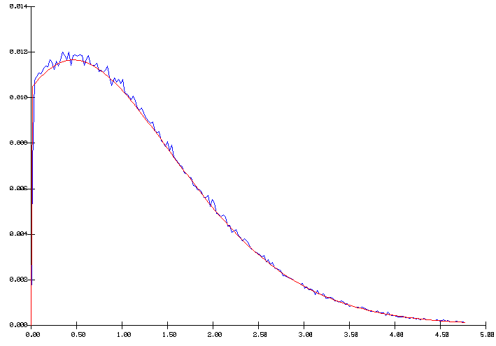
Figure 1 - Poisson distribution with a mean of 1
In figure 1, we can distinguish two curves: the smooth curve is the targeted distribution while the seesaw curve was obtained by compiling the results of 100 000 random values based on that distribution. The results indicate that a simple and fast random number generator [11] is acceptable.
ANALYSIS OF RISK ASSESSMENT
Let´s now assume, still using the previous example of the 300 kA cell, that the anode voltage drop and anode panel heat loss were determined by an anode model with an accuracy of 5%. These two cell parameters were thus assigned the following error margins:
| · Anode voltage drop (mV) | 300 ± 15 | ||
| · Anode panel heat loss (kW) | 235 ± 12 |
The impact of these error margins on the expected operating cell characteristics was determined first individually then combined.
Anode voltage drop
In the first run, all the input parameters were defined as they appear in Table II except for the anode voltage drop which was defined as a ramp probability distribution between 285 to 315 mV (see figure 2). The Monte Carlo analysis was run for 100 000 cycles using the ACD as the selected output variable.
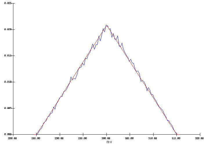
Figure 2: Input ramp distribution of the anode drop
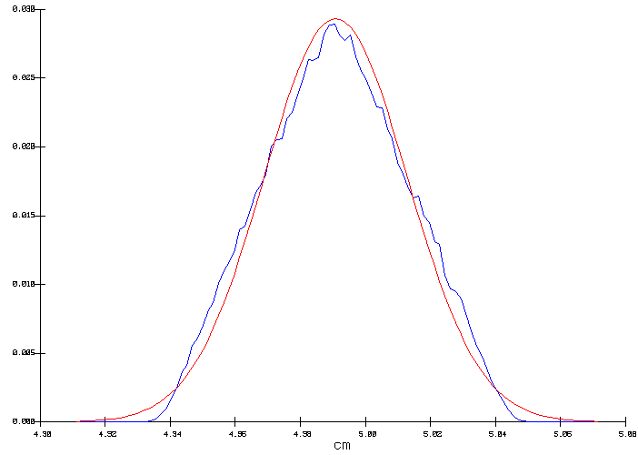
Figure 3: Output distribution of the ACD
Figure 3 shows two curves: the seesaw curve is the obtained output distribution while the smooth curve is the normal distribution that corresponds to the computed output distribution mean and standard deviation of 4.996 and 0.0334 cm, respectively.
In this example, the input ramp distribution of the anode voltage drop (figure 2) was reproduced in the resulting output ACD distribution (figure 3). This is explained by the fact that since the input parameters defined a constant heat loss, the ACD needs to be adjusted in order to compensate for the heat not produced in the anodes in order to maintain the internal heat constant. In the context of a cell designed at the edge of magnetic stability, this error margin of 0.9 mm on the ACD could well make the difference between a stable or an unstable cell design.
Anode panel heat loss
In the second run, a normal probability distribution was assigned for the anode panel heat loss (see figure 4). The mean was set to 235 kW and a standard deviation was set to 6 kW. The ACD was set to 4.9951 and the cell temperature was selected as the output variable.
The output distribution is a true normal distribution characterized by a mean of 975 °C and a standard deviation of 0.476 °C (figure 5). This time, the internal heat is constant, so in order to maintain the heat loss constant, the cell superheat had to be adjusted to compensate for the heat not dissipated by the anode panel. As we can see in figure 6, this has a significant impact on the corresponding average freeze thickness at the bath level to be expected from that cell design.
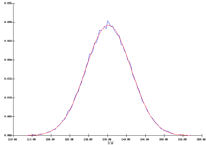
Figure 4: Input normal distribution of the anode panel heat loss
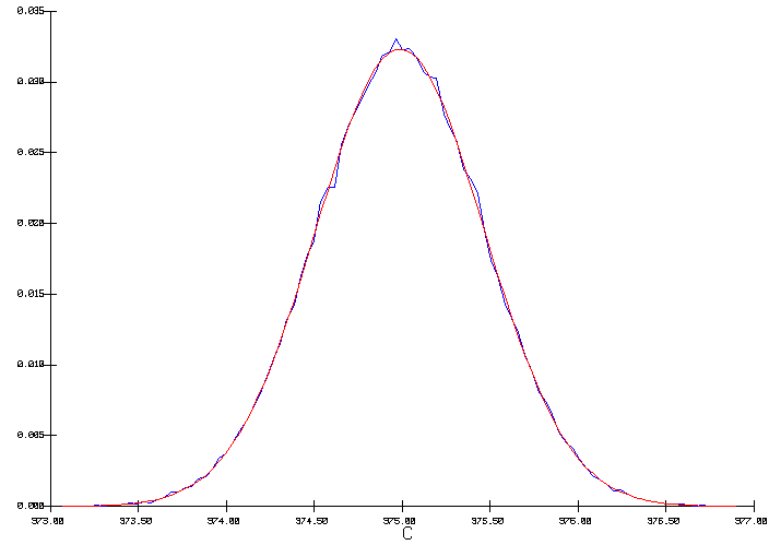
Figure 5: Output distribution of the cell temperature
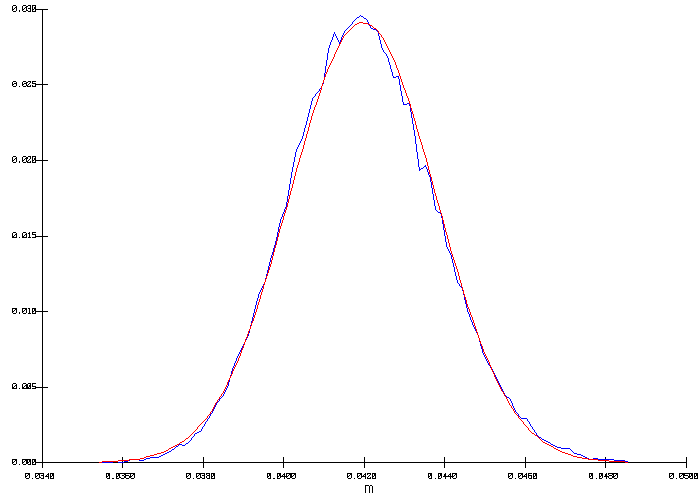
Figure 6: Corresponding distribution for the freeze thickness at bath level
Combination of voltage drop and anode panel heat loss
In the third run, the effect of both margins of error were combined. Notice first that in the first run, the distribution on the anode voltage drop had an influence on the internal heat and by selecting ACD as output variable, the cell internal heat was kept constant. In the second run, the distribution on the anode panel heat loss had an influence on the heat loss and by selecting the cell operating temperature as output variable, the cell heat loss (and the corresponding internal heat) was kept constant. This mean that in both cases the cell voltage was kept constant at 4.27 V.
It is desirable to perform analysis of risk assessment at a constant cell voltage, since it is representative of the real cell operational mode, but this would not occur automatically in this third run since the internal heat and the heat loss will both vary.
To force an analysis at constant cell voltage, the outcome value of the anode voltage drop (from the ramp probability distribution of figure 2) must be used to compute an ACD input value that corresponds to the target cell voltage of 4.27 Volts (figure 3). Then, the normal distribution is used to define the anode panel heat loss (figure 4). Again, the temperature is chosen as output variable.
This third run produced a temperature output distribution identical to the second run (figure 5) indicating that at constant cell voltage, the impact of those two margins of error are not strongly interacting.
Nevertheless, considering the combined impact of both input distributions, forcing a constant cell voltage does not mean forcing a constant internal heat as indicated by the obtained distribution for the cell internal heat/heat loss characterized by a mean of 623.2 kW an a standard deviation of 0.267 kW.
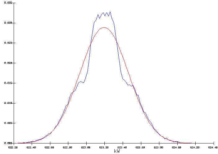
Figure 7: Output distribution of the cell internal heat
A more complicated case study involving more input distributions would obviously result in more complex output distributions having larger standard deviations.
CONCLUSIONS
An enhanced computer program was developed to simulate the steady state behavior of an aluminum reduction cell more flexibly. The program can be used to perform Monte Carlo simulation where the user can assign probability functions to cell input parameters and the program calculates the distribution of the output parameters. The calculated distribution(s) can be of value in the analysis of risk assessment of new or retrofitted cell design.
Examples of practical applications were presented to demonstrate the flexibility of the program.
REFERENCES