FURTHER IMPROVEMENT OF ALUMINIUM REDUCTION CELL

RESISTANCE SLOPE CALCULATION

Marc Dupuis

GéniSim Inc.

3111 Alger St.

Jonquière, Québec, Canada G7S 2M9

marc.dupuis@genisim.com

ABSTRACT

Assuming that the cell is not excessively mucked and hence that the evolution of

the cell resistance is mostly dictated by the evolution of the concentration of the

dissolved alumina in the bath, it is fair to say that calculating the slope of that cell

resistance can now be considered as an exact science.

During the underfeeding regime from the lean side of the cell voltage vs alumina

concentration curve, the gradual increase of the slope of the cell voltage is well known

and the added bubble and MHD driven cell voltage noise is very well known as well.

Hence finding the optimal numerical algorithm to filter out that noise and

calculating the current noise free cell resistance slope is a strait forward proposal. In the

past the limited C.P.U. power of cell controller may have prevented the usage of such an

algorithm, but this is no longer a limitation.

INTRODUCTION

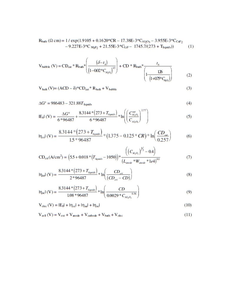
In absence of excessive muck, we can assume that the equations used in [1] and

presented below represent well the evolution of the bath resistivity, bath resistance, cell

over-potentials etc. and hence can well represent the evolution of the cell resistance slope

during an underfeeding alumina feeding regime that would lead to the cell having an

anode effect if the cell controller doesn’t activate the overfeeding alumina feeding in

time.

The equations above or very similar ones presented in [2] can be used to calculate

the evolution of the cell voltage as the concentration of dissolved alumina gradually

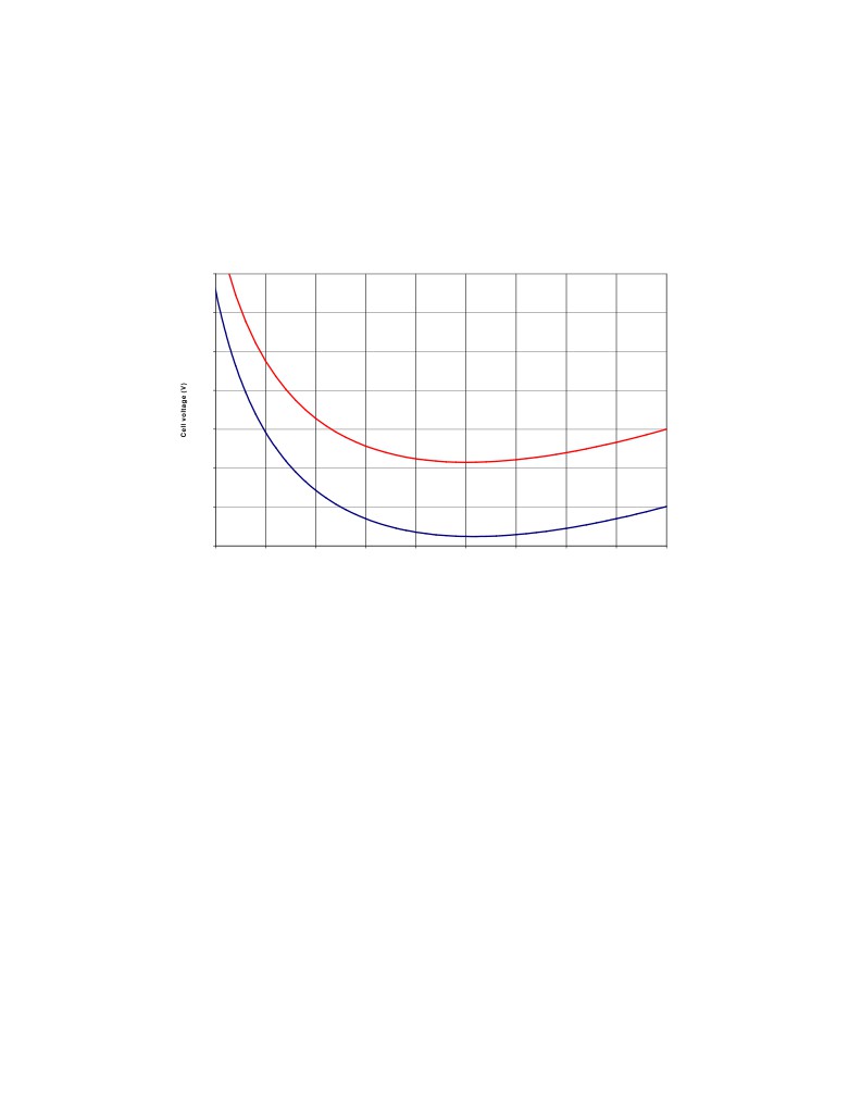
increases in the bath. Figure 1 presents two such curves for two different values of the

ACD.

In the flat section around 4% of dissolved alumina concentration, the cell voltage

reaches a minimum. In that region, a little variation of the concentration of dissolved

alumina in the bath is not affecting the cell voltage, which is why ACD is typically

adjusted at the end of the overfeeding regime when the concentration of dissolved

alumina is assumed to be around that value.

It is very important to know that those equations are not accounting for the impact

of dispersed alumina and muck formation on the cell voltage. This is why the voltage

increase on the right or rich alumina concentration side of the curves is underestimated.

Cell voltage vs concentration of dissolved alumina

4.290

4.270

4.250

4.230

4.210

4.190

4.170

4.150

1.5

2.5

3.5

4.5

5.5

Concentration of dissolved alumina (%)

Figure 1: Cell voltage vs concentration of dissolved alumina

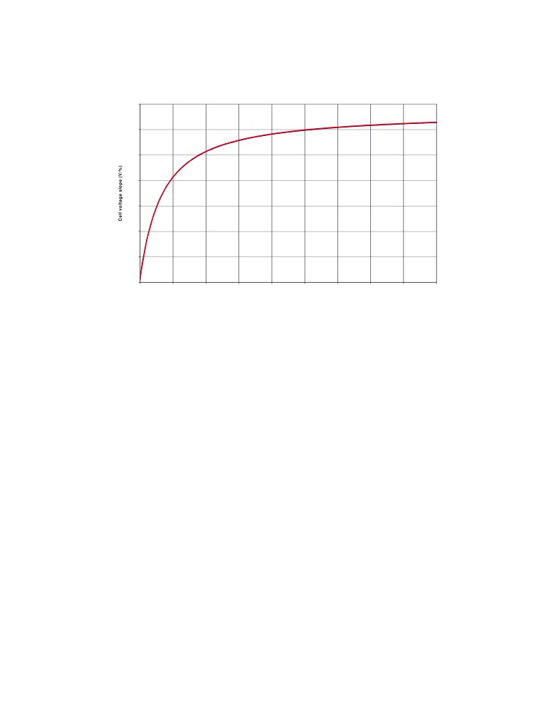
Of course as illustrated in Figure

2, the first derivatives of the two curves

presented in Figure 1 are identical hence independent of ACD. Furthermore, close to

anode effect dissolved alumina concentrations, the variation of the cell voltage due to the

variation of the ACD is completely negligible as compared to the variation of the cell

voltage due to the variation of the concentration of dissolved alumina.

Cell voltage slope vs concentration of dissolved alumina

0.05

-0.05

-0.1

-0.15

-0.2

-0.25

-0.3

1.5

2.5

3.5

4.5

5.5

Concentration of dissolved alumina (%)

Figure 2: Slope of the cell voltage vs concentration of dissolved alumina

So assuming that during the underfeeding regime the rate of decrease of the

concentration of dissolved alumina is linear, there a direct relationship between the slope

(or first derivative vs time) of the cell voltage and the concentration of dissolved alumina

in the cell.

In typical continuous tracking control logic, a given value of the cell resistance

slope is used to trigger the alumina overfeeding regime before the anode effect occurs. In

the new more innovative In Situ [3] alumina feeding control logic, the value of the slope

of the normalized cell voltage is used to estimate the dissolved alumina concentration

and than the normalized cell voltage is used to estimate the ACD.

Notice that if the cell is very mucky, the rate of decrease of the concentration is

probably not linear even close to the anode effect dissolved alumina concentration.

Furthermore, the cell voltage may also be affected by the presence of the muck even on

the left or the lean side of the curve.

SMOOTHING/FITTING THE CELL NORMALIZED VOLTAGE

OR CELL PSEUDO RESISTANCE

So the key to modern alumina feeding control logics and their associated very

good operational results of 95-96% current efficiency and 0.05 or less anode effect per

pot per day is the controller ability to calculate the cell pseudo resistance or cell

normalized voltage slope despite the noise in the amperage and voltage signals and keep

operating the cell on the lean side of the slope in order to avoid muck formation.

Because the cell amperage is fluctuating, the cell voltage is not directly used in

control logic algorithms. The normalized cell voltage or the cell pseudo resistance is used

instead. The definition of the cell pseudo resistance and the cell normalized voltage are

presented below:

Ω_cell = (V_cell - BEMF ) / I

(12)

V_cellnorrm = (V_cell - BEMF ) / I * I_nom + BEMF

(13)

Where:

BEMF is the extrapolated voltage at zero amperage usually set to 1.65 (V)

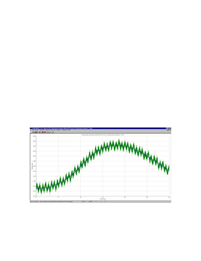
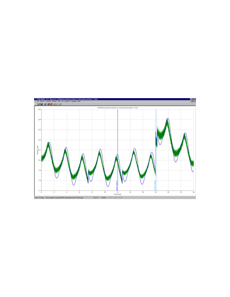
Both variables are free of noise from amperage fluctuation (see [4] for more

details) but still contain noise from the bubble release and the MHD driven bath-metal

interface wave motion. As an example, Figure 3 presents cell voltage data generated by a

cell simulator [1] both before adding the bubble and MHD fluctuation and after their

addition. At the sampling frequency of 10 Hz, it is quite easy to distinguish the MHD

wave gradual evolution superimposed on the much slower variation mostly due to the

slow evolution (for that time scale) of the dissolved alumina concentration. As opposite,

the impact of the bubble still looks like white noise at that sampling frequency.

Figure 3: Evolution of the cell pseudo resistance with and without noise

At an even higher sampling frequency and a smaller time scale, even the green

curve would look like a smoothly evolving curve but this is not required. The point is to

process the green curve data in order to calculate as accurately as possible the slope of

the blue curve.

First numerical scheme requiring the bare minimum computer resources

The first numerical scheme that will be presented here has already been presented in [5];

it requires the bare minimum computer resources typical of the type of numerical scheme

developed about 25 to 30 year ago.

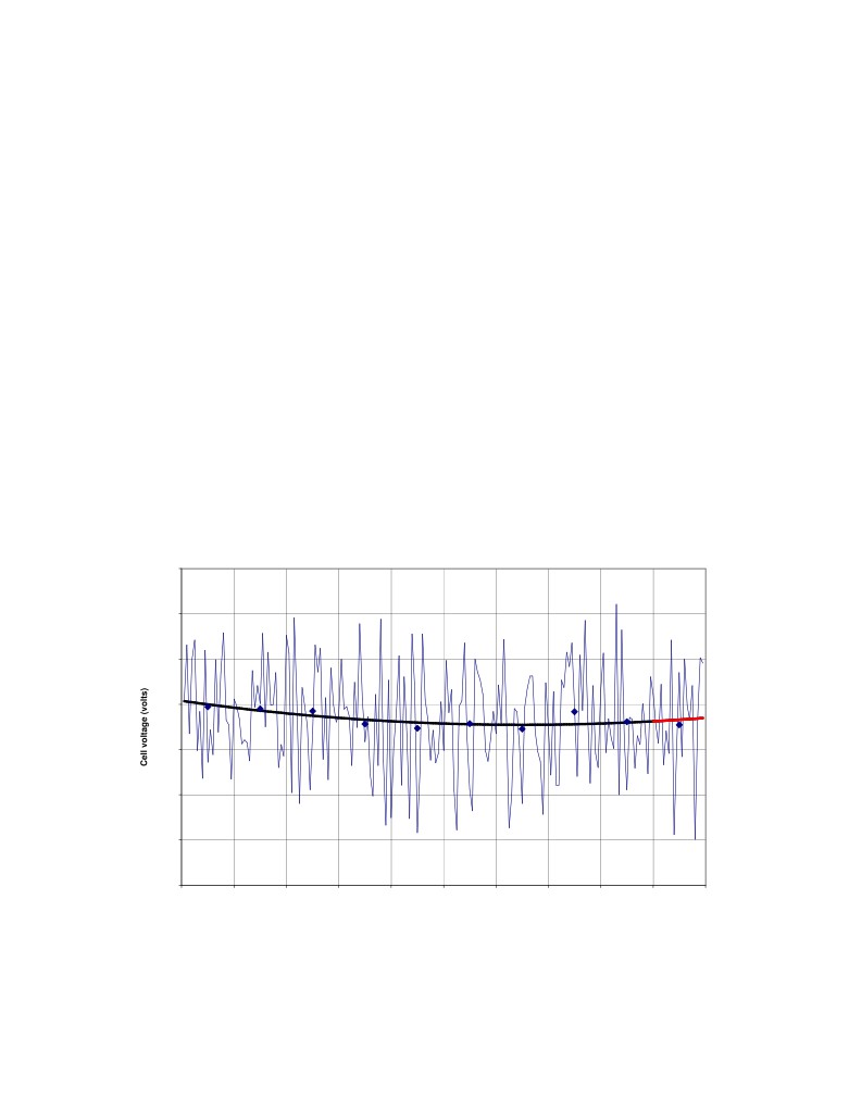
The cell voltage is sampled every 6 seconds or at a frequency of 0.16667 Hz and

averaged every 2 minutes. At each of those 2 minutes cycles, the last ten 2 minutes

averaged value datapoints are fitted using quadratic root mean square (RMS). The slope

of the fitted parabola at time zero is compared against the trigger slope value to decide if

it is time to shift from underfeeding to overfeeding mode (see Figure 4).

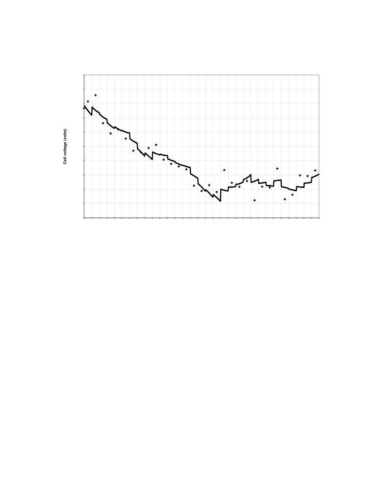
Figure 5 presents the successive addition of the red curve sections of Figure 4. Time 0 of

Figure 4 is time 80 of Figure 5, so the red curve section of Figure 4 is the last curve

section of figure 5. As discussed in [5], the calculated slope is still very noisy, the slope

calculated using linear RMS instead with the same 10 datapoints is less noisy but it

represents the best fit of the slope 10 minutes in the past. Clearly those schemes are not

good enough, they lead to either many escaped anode effects if the trigger slope is set to

high or too many false positives leading to slugging problems if the trigger slope is set to

low.

Voltage noise filtration

4.426

4.424

4.422

4.42

4.418

4.416

4.414

4.412

-20

-18

-16

-14

-12

-10

-8

-6

-4

-2

Time (minutes)

Figure 4: Quadratic RMS fit using ten 2 minutes averaged value datapoints

Voltage noise filtration

4.423

4.4225

4.422

4.4215

4.421

4.4205

4.42

4.4195

4.419

4.4185

4.418

Time (minutes)

Figure 5: Successive addition of the red curve sections of Figure 4

Second numerical scheme requiring more computer resources

Gradually as years passed, it became possible to use numerical scheme requiring

more computer resources. The second set of numerical schemes presented here is

presented in [4].

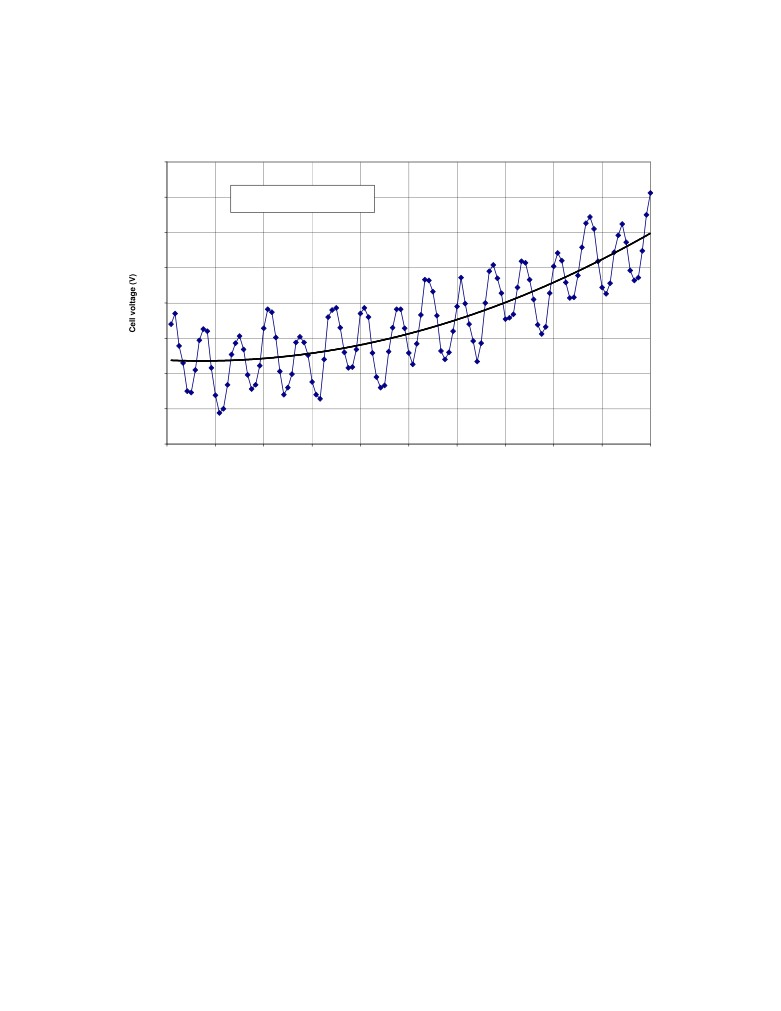
The cell voltage is sampled at a frequency of 10 Hz and averaged every 5

seconds. At each of those 5 seconds cycles, the last one hundred and twenty (120) 5

seconds averaged value datapoints are fitted using RMS. The resulting parabolic fit is

presented in Figure 6.

Quadratic root mean square fit of normalized cell voltage

4.13

y = 0.000210x² - 0.000301x + 4.101891

4.125

R² = 0.650806

4.12

4.115

4.11

4.105

4.1

4.095

4.09

Time (min)

Figure 6: Quadratic RMS fit using one hundred and twenty (120) 5 seconds

averaged value datapoints

Performing a 120 datapoints quadratic RMS fit every 5 seconds is obviously far

more demanding on the cell controller CPU than performing a 10 datapoints quadratic

RMS fit every 2 minutes but, as presented in Figure 7, there is far less noise left in the

slope estimate.

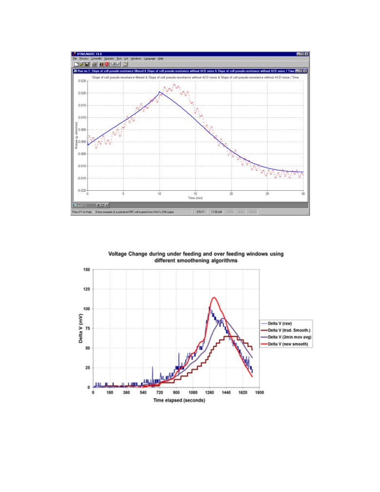
Yet, there is clearly some noise left as compared to the noise free fit calculated in

[6]. Figure 8 is a reproduction of Figure 4 in [6]. There is no delay in the slope estimate

and there is an overshoot after the change of feeding regime which are both signatures of

quadratic RMS fitting. The only difference between the red curve of Figure 7 and the red

curve of Figure 8 is the lack of noise in the red curve of Figure 8.

Optimum noise filtration numerical scheme

Clearly these days, considering the very low cost of hardware and the industry

desire to continue to reduce anode effect frequency, there should be no hardware related

limitations when selecting the noise filtration numerical scheme and hence, the one

selected should be the one the producing the optimal results.

For the purpose of this work, the optimal filtration numerical scheme would be

one that produces a filtered slope with no visible noise. Figure 9 presents the raw noisy

cell pseudo resistance in green and the optimally filtrated cell pseudo resistance in blue.

As can be seen, the blue curve is 100% noise free.

Figure 9: Raw noisy and filtrated cell pseudo resistance

The blue curve do overshoot the green curve each time the feeding regime is

changed which again is typical of quadratic RMS fit. As for the first two noise filtration

numerical scheme, this third “optimal” one consists of sampling the cell voltage at a

given frequency, averaging the sampled value to generate datapoints and fitting a given

number of those datapoints using quadratic RMS.

It can be noticed that the numerical scheme used generates a new slope

calculation each time a new datapoint is generated. Obviously with this third numerical

scheme, a new slope calculation is generated at a significant higher frequency that once

every 5 seconds and far more that 120 datapoints are fitted, the optimum number.

It can also be noticed that the numerical scheme used can cope with the

discontinuity in the curve produced by moving the anode bridge. Four such bridge

motions occur during the displayed 24 hours time frame cell evolution presented in

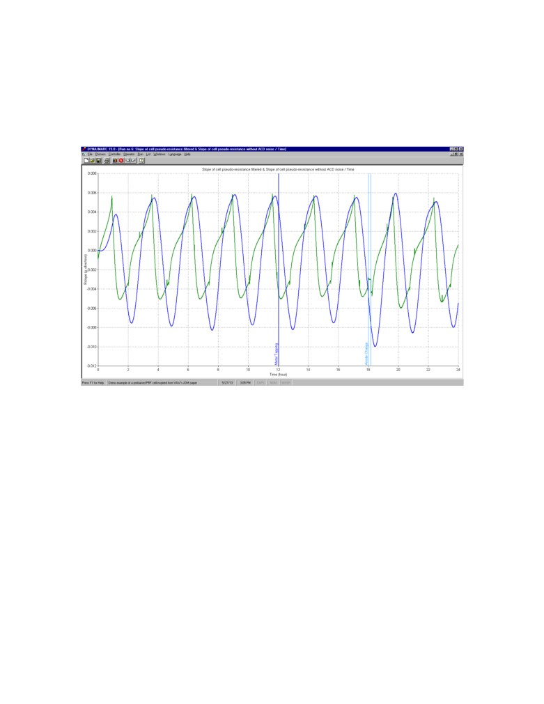
Figure 9. Figure 10 presents the comparison between the noise free cell pseudo resistance

slope evolution in green and the filtered pseudo resistance slope evolution in blue.

Figure 10: Quadratic root mean square fit of the pseudo resistance slope

As desired, the filtered pseudo resistance slope evolution curve is 100% noise free

and is not lagging the noise free curve toward the end of underfeeding. The fit is

obviously not perfect but can be considered optimum as it is fulfilling the requirements

for cell control needs.

CONCLUSIONS

Assuming that the cell is not excessively mucked and hence that the evolution of

the cell resistance is mostly dictated by the evolution of the concentration of the

dissolved alumina in the bath, the evolution of the slope of that cell resistance vs the

dissolved alumina concentration is following an established path.

Hence during the underfeeding regime from the lean side of the cell voltage vs

alumina concentration curve, the gradual increase of the slope of the cell voltage is well

known and the added bubble and MHD driven cell voltage noise is very well known as

well.

It follows that in those circumstances calculating the slope of that noisy cell

resistance can now be considered as an exact science. Hence finding the optimal

numerical algorithm to filter out that noise and calculating the current noise free cell

resistance slope was a straightforward proposal.

That optimal numerical algorithm requires more computer resources than those

currently used in the industry but considering the very low cost of hardware and the

industry desire to continue to reduce anode effect frequency, there clearly should be no

hardware related limitations when selecting the noise filtration numerical scheme.

REFERENCES

(1) DUPUIS, M. and COTE, H., 2012.

Dyna/Marc Version 14 User's Guide.

(2) HAUPIN, W., 1998.

Interpreting the components of cell voltage, Light Metals, TMS, p. 531-537.

(3) SCHNELLER, M. C., 2009.

In Situ alumina feed control, JOM, Vol. 61 No. 11, p. 26-29.

(4) DUPUIS, M. AND SCHNELLER, M. C., 2011.

Testing In Situ Aluminium Cell Control With the Dyna/Marc Cell Simulator, Light

Metals, COM

(5) DUPUIS, M., 2007.

Cell voltage noise removal and cell voltage (or resistance) slope calculation, 12th

IFAC Symposium on Automation in Mining, Mineral and Metal Processing (IFAC

MMM'07)

(6) ZAROUNI, A. and Al., 20012.

Achieving low greenhouse gases emission with DUBAL’s high amperage cell

technology, ICSOBA.